Analog-to-digital conversion, or ADC, is a fundamental part of the digital audio workflow. Audio interfaces are dedicated devices that specialize in ADC. Although there are various approaches to ADC, they all rely on the process of ‘sampling’. In this article, we’ll look at the basics of sampling, how it works, and the key parameters associated with it.

In this article we’ll look at:

• What is ADC and why do we need it?
• How ADC sampling works
  • Sampling rate
  • Bit depth
• Implications of ADC parameters
  • Dynamic range
  • Quantization distortion
  • Processing burden
  • Latency
• Conclusion
• FAQs

What is ADC and why do we need it?

In a digital audio workflow, analog-to-digital conversion (ADC) is the process of converting an analog audio signal into a digital audio signal.

It’s a fundamental part of the digital audio workflow and is necessary for working with digital audio, given the way that sound manifests in our natural world.

Sound appears as continuous waveforms in the world around us. When generated through voice or physical instruments (whether directly or through amplified speakers), sound travels through the air to reach our ears or other listening devices.

Being made up of continuous waves, sound generated in this way is an analog signal.

Computers, on the other hand, operate in a digital environment. They require information to be in a discrete, numeric format.

Since computers are integral to the digital audio process, natural (analog) sound needs to be converted into a discrete (digital) format to be processed. This is what ADC does.

Audio interfaces are devices that are dedicated to ADC (amongst other things). They receive analog sound in the form of continuous, analog audio signals (through microphones or instrument inputs) and use ADC to convert this to digital audio signals for further processing.

How ADC sampling works

There are various approaches to ADC, each with its own strengths and weaknesses depending on the application. But underlying all of them is the process of sampling.

The basic approach to sampling is straightforward:

1. For an incoming analog signal (waveform), take periodic ‘snapshots’ over time (i.e., samples)
2. For each sample, take a measurement of the amplitude (or loudness) of the analog waveform
3. Record each measurement, for each sample, using a (binary) number system to a desired level of precision

There are two key parameters in the sampling process: the sampling rate and the bit depth.

Sampling rate

As we’ve discussed, the sound coming from an instrument or voice is an analog signal.

This can be represented as a continuous waveform with a vertical axis that indicates its amplitude (how loud the sound is) and a horizontal axis that indicates time. The more peaks and troughs (ups and downs) in the waveform over a given period of time, the higher the sound’s frequency (pitch).

So, how do you convert a waveform from something that’s continuous into something that’s discrete?

A simple approach is to take snapshots, or samples, of the waveform at discrete points in time.

Figure 1 shows an example of a continuous (analog) waveform. The vertical axis represents the amplitude of the waveform and the horizontal axis represents time.

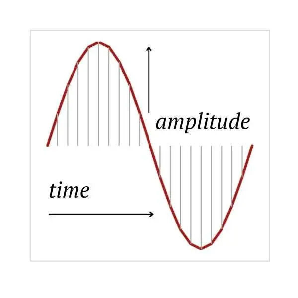
The vertical lines in the waveform indicate points in time at which samples occur—at each sample, a measurement of amplitude can be taken (the level at which the vertical line meets the waveform).

An obvious question that you may ask is “how many samples should you take?”. The answer depends on a number of factors, but all else equal, the more samples the better.

Figure 2 shows the same waveform with the same number of samples being taken (left-hand chart), and also when more frequent samples are being taken (right-hand chart)—when more samples are taken, a better representation of the original (analog) waveform is possible.

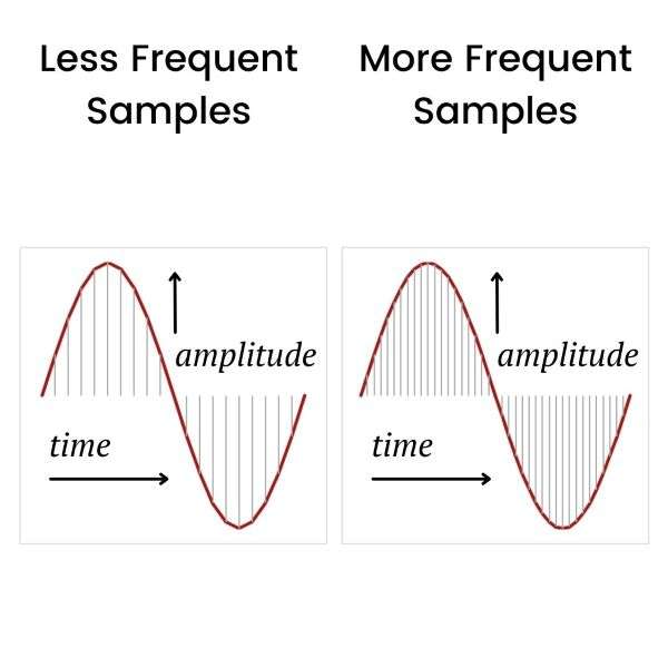
In ADC, the number of samples of an analog waveform taken per second is known as the sampling rate.

The Nyquist rate

Modern audio interfaces work with sampling rates from 44.1 kHz to 192 kHz.

Hz is an abbreviation for hertz, referring to the number of cycles per second (or in our case, samples per second). So, 44.1 kHz refers to a sampling rate of 44,100 samples per second.

As it happens, there’s a theoretical formula called the Nyquist-Shannon sampling theorem that suggests you should use a sampling rate that’s at least twice the (highest) frequency of the signal you’re sampling. This is sometimes referred to as the Nyquist rate.

Oversampling

So, a 44.1 kHz sampling rate is enough to capture sound frequencies up to around 22 kHz. This is in line with the normal frequency range of human hearing, which is generally from 20 Hz to 20 kHz.

44.1 kHz is also the sampling rate used for capturing sound on CDs.

But many audio interfaces use sampling rates much higher than 44.1 kHz (up to 192 kHz, for instance)—why?

Such frequencies go far beyond what’s necessary for human hearing.

This practice of sampling at higher rates than necessary is referred to as oversampling. And one of the key reasons for oversampling is to minimize aliasing.

Aliasing

Aliasing can arise when sampling is done at a rate that’s below the Nyquist rate (twice the highest frequency that’s present in the original analog signal).

When aliasing occurs, it results in unwanted frequencies being produced in the range of human hearing, i.e., an undesirable outcome for an audio production process.

But if the frequency range of human hearing only goes up to around 20 kHz, isn’t a CD-quality sampling rate of 44.1 kHz sufficient to avoid aliasing?

The answer in many situations is no.

Although humans can’t hear it, many musical instruments (and other sounds in the natural world) produce frequencies that are much higher than 20 kHz.

According to measurements taken by James Boyk, for instance, a musician and former lecturer at the California Institute of Technology, many musical instruments routinely produce frequencies above 40 kHz. And some instruments produce much higher frequencies, e.g., trumpets up to 80 kHz and cymbals more than 100 kHz.

The oversampling used by some audio interfaces, therefore, attempts to minimize the impact of aliasing from the very high frequencies produced by musical instruments and other sounds.

Keep in mind that the actual frequencies received by the audio interface will depend on the degree of frequency filtering that occurs via the interface’s inputs (microphone or line signals), but the possibility of high input frequencies still exists.

Bit depth

Now that we’ve looked at how samples of continuous (analog) waveforms are taken, we need a way of recording each sample.

Figure 3 shows two ways of recording samples of a waveform.

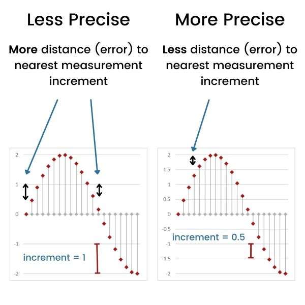
In the graph on the left of Figure 3, the levels (or amplitudes, shown by horizontal lines) of the waveform are measured in increments of 1. In the graph on the right, the amplitudes are measured in increments of 0.5.

When using increments of 1 for each sample (vertical line), the amplitude measurement can only be recorded to the nearest whole number (i.e., 1, 2, etc.). So, the distance between the actual amplitude (which may be, say, 1.6) and the recorded amplitude (which would be the nearest whole number, i.e., 2) would be up to 0.5 in size (in our example it would be 2-1.6=0.4).

Quantization error

The distances between actual and recorded amplitudes can introduce a degree of error in the way that the analog signal is measured during the digitization process.

As we’ve seen, in the graph on the left of Figure 3 this error can be up to 0.5 in size with each sample.

When we use measurement increments of 0.5, however, as in the graph on the right of Figure 3, the size of the possible error per sample reduces.

Here, the distance between the actual amplitude (say, 1.6) and the recorded amplitude (which would be the nearest ½ number, ie. 1.5) would only be up to 0.25 in size (in our example it would be 1.6-1.5=0.1).

So, the possible degree of error in recording each sample reduces when we use smaller increments.

We can, therefore, be more precise in recording our sample amplitude measurements when we use smaller increments.

This process of recording sample measures by using the nearest available measurement increments is called quantization. And the error that’s caused by the differences between actual and recorded measurements is the quantization error.

Sample resolution

When you use smaller increments to record your measurements, you need a larger quantity of numbers to capture a given amplitude range.

Consider an amplitude range of 0–100, for instance. If we use whole increments, we have 101 possible numbers to take our measurements with (i.e., 0, 1, 2, …, 99, 100).

But if we use 0.5 increments, we have 201 numbers to take measurements with (i.e., 0, 0.5, 1.0, …, 99.5, 100).

Recall that digital computer systems are based on binary numbers, i.e., where all numbers are represented by 0s and 1s. So, if we want to take more precise measurements using a binary number system, and reduce the quantization error, we need to have a larger quantity of (binary) numbers available to use.

This is why bit depth plays an important role.

In a binary system, the bit depth is the number of bits used for recording each measurement in a sample, which in turn determines the total quantum of numbers available to us—the larger the bit depth, the more numbers we can use and the more precise we can be in our measurements.

If we use 16-bit numbers for our sample measurements, for instance, we have a total of 65,536 (=2¹⁶) unique values at our disposal.

But if we use 24-bit numbers, we have 16,777,216 (=2²⁴) unique numbers to work with—we can take far more precise measurements using 24-bit numbers rather than 16-bit numbers!

The bit depth is sometimes referred to as the resolution of the digital sample.

This term has intuitive appeal, as a higher bit depth results in more precise measurements, which many people would associate with a higher resolution.

While CD-quality sound has a 16-bit resolution, most modern audio interfaces offer ADCs with a 24-bit resolution. This offers more precise sampling measurements for audio production needs.

Implications of ADC parameters

As we’ve seen, the sampling rate and the bit depth are two important parameters in the ADC process.

But what are the implications of choosing different values for these parameters?

Let’s consider these.

Dynamic range

From our discussion on bit depth, we know that under a binary system, 16-bit numbers give us 65,536 (=2¹⁶) discrete levels to work with. Similarly, 24-bit numbers give us 16,777,216 (=2²⁴) discrete levels to work with.

More generally, when we use n-bit binary numbers to digitize an analog sample, we’ll have 2ⁿ discrete levels to work with.

And as we know, the more numbers that we have to work with, i.e., the larger the bit depth, the more precisely we can record measurements during digitization.

But other than precision, a larger bit depth also translates to a larger dynamic range.

The dynamic range is the ratio of the loudest possible sound to the quietest sound in an audio signal.

These ratios can be very large, so the dynamic range is measured in decibels (dB) which is a logarithmic scale.

The dynamic range is related to the bit depth as follows: For a bit depth of n, the dynamic range is 6n dB.

So, when we use a bit depth of 16 bits, the dynamic range is 96 dB. When we use 24 bits, the dynamic range increases to 144 dB.

These are theoretical maximum values, so in practice the dynamic range may be lower due to noise produced by circuitry in and around the ADC.

Nevertheless, a higher dynamic range is beneficial as it means there’s more scope for differentiating loud and soft sounds. This allows for higher signal-to-noise ratios in the audio recording process.

Quantization distortion

Earlier, we mentioned the quantization error that arises during the sampling process. The bigger the differences between the actual and recorded measurements of analog samples, the larger the quantization error.

The quantization error produces a certain level of distortion in the digitized audio signal. This is referred to as the quantization distortion.

There’s a theoretical relationship between the bit depth and the quantization distortion: For a bit depth of n, the quantization distortion is 100/2ⁿ percent.

So, for a bit depth of 16 bits, the quantization distortion is 0.0015% (=100/2¹⁶ percent). When using a bit depth of 24 bits, however, the quantization distortion reduces to less than 0.00001%.

Again, these are theoretical (minimum) values, and in practice, the distortion is likely to be higher.

Processing burden

Given the implications for precision, dynamic range, and quantization distortion, it may seem a straightforward decision to prefer a larger bit depth over a smaller one. So, 24-bit sampling would always be preferred to 16-bit sampling, right?

Not always.

It’s true that a larger bit depth is beneficial, but it comes at a cost.

A computer’s processor has to work harder for a digitization process that uses a larger bit depth.

This may adversely affect your recording outcomes if your computer’s processing capacity is insufficient for the various tasks it’s working on.

Latency

Latency refers to the time taken for an audio signal to travel through an audio workflow. If it becomes too large, it becomes noticeable and impacts the recording process.

One of the ways of controlling latency in your digital audio workflow is to reduce the buffers being used in your DAW software. These buffers are for temporary memory storage and help ease the burden on a computer’s processing capacity.

The higher the buffer setting, the lower the burden on a computer’s processor but the worse the latency, and vice-versa.

As we’ve seen, however, a higher bit depth adds to the processing burden of a computer system.

In a computer system without much spare processing capacity, a higher bit depth may limit the computing power available for reducing latency. Higher buffer settings may be required as a result.

So, an additional implication of choosing a higher bit depth is that it may lead to increased latency issues.

Conclusion

ADC is the process of converting analog audio signals to a digital form and is a fundamental part of the digital audio workflow.

Audio interfaces are specialized devices for ADC.

While ADC methods used by audio interfaces can vary, they all rely on the process of sampling.

The sampling process consists of:

• Sampling an analog audio signal at discrete points in time
• Taking a measurement of the signal’s amplitude at each sample
• Recording the measurement in a binary (computer-friendly) format to a desired level of precision

Two of the key parameters in this process are the sampling rate and the bit depth.

The sampling rate is the number of samples taken per second. The higher the sampling rate, the better the digital capture of an analog audio signal.

According to Nyquist’s theorem, the sampling rate should be at least twice the frequency of the highest frequency component in the original analog signal. This helps to ensure that possible distortions due to aliasing are minimized.

Many audio interfaces offer sampling rates as high as 192 kHz for this reason—although human hearing doesn’t go much beyond 20 kHz, certain musical sounds can have frequencies above 100 kHz.

The bit depth refers to the number of bits used for recording each sample measurement under a binary system. The higher the bit depth, the more precision in the recorded measurements.

A higher bit also increases the (maximum possible) dynamic range of the processed digital sound and reduces the (minimum possible) level of quantization distortion.

Many audio interfaces offer bit depths of 24 bits—this allows for a dynamic range of up to 144 dB and a quantization distortion below 0.00001%.

But, while a higher bit depth is beneficial, it comes at the cost of increased demands on computer processing power—if this becomes too high, it may lead to issues such as latency, due to insufficient spare processing power being available.

ADC is necessary for a digital audio workflow and audio interfaces offer powerful ADC capabilities. By selecting the best ADC parameters for your system, you can achieve your desired balance between output quality and processing ability for your digital audio setup.

FAQs